Some notes about Preimage-Sampleable Trapdoor Function, note structure is heavily relying on dwu4’s course, with some other readings in GPV04, MP11 and Pei11.

Some notes about lattice-based ZKP from Lyu12, BDLOP16, LS18 about reject sampling, lattice-based commitment, etc.

All the info comes from [BDIR19] and [MPSW20]

First Attempt…

Fix a $(n,m)$ local leakage function $\vec{L}$ and let $\vec{\ell} \in \left(\set{0,1}^m\right)^n$ be a leakage value. Let $L_i^{-1} (\ell_i) \subseteq \mathbb{F}$ be the subset of $i$-th party’s shares such that the leakage function $L_i$ outputs $l_i \in \set{0,1}^m$.

$s_i \in L_i^{-1}(\ell_i) \iff L_i(s_i) = \ell_i$.

Therefore, for leakage function $\vec{L}$ we have leakage $\vec{\ell}$ if and only if the set of secret shares $\set{\vec{s}}$ belongs to the set
$$
\vec{L}^{-1}(\vec{\ell}) := L_1^{-1}(\ell_1) \times \cdots \times L_n^{-1}(\ell_n)
$$
Thus the probability of leakage being $\vec{\ell}$ conditioned on the secret being $s^{(0)}$ is
$$
\frac{1}{|\mathbb{F}|^k} \cdot \left| s^{(0)} \cdot \vec{v} + \langle G \rangle \cap \vec{L}^{-1}(\vec{\ell}) \right|.
$$
We can formulate the probability of leakage being $\vec{\ell}$ conditioned on the secret being $s^{(1)}$ similarly, and give the statistical distance
$$
\Delta(\vec{L}(s^{(0)}), \vec{L}(s^{(1)})) = \frac{1}{2} \cdot \frac{1}{|\mathbb{F}|^k} \sum_{\vec{\ell} \in \left(\set{0, 1}^m\right)^n} \Bigg| \left| s^{(0)} \cdot \vec{v} + \langle G \rangle \cap \vec{L}^{-1}(\vec{\ell}) \right| - \left| s^{(1)} \cdot \vec{v} + \langle G \rangle \cap \vec{L}^{-1}(\vec{\ell}) \right| \Bigg|.
$$

(nope, it is hard to bound…)

All the info comes from [BDIR19] and [MPSW20]

Massey Secret-Sharing Scheme

Let $\mathbb{F}$ be a finite field, a linear code $C$ over $\mathbb{F}$ of length $n+1$ and rank $k + 1$ is a $(k+1)$-dimension vector subspace of $\mathbb{F}^{n+1}$, referred to as $[n+1,k+1]_{\mathbb{F}}$ code.

Generator matrix $G\in \mathbb{F}^{(k+1)\times (n+1)}$ of $[n+1,k+1]_\mathbb{F}$ linear code $C$ ensures that $\forall c \in C$ exists $\vec{\boldsymbol{a}}\in \mathbb{F}^{k+1}$ such that $c \equiv\vec{\boldsymbol{a}}\cdot G$.

The rowspan of $G$ is represented as $\langle G \rangle$, it is also the code generated by $G$. In standard form $G = [I_{k+1}|P]$ where $P$ is the parity check matrix.

Write $C \subseteq \mathbb{F}^{n+1}$ be the linear code generated by $G$, the dual code of $C$ is written as $C^\bot \subseteq \mathbb{F}^{n+1}$, which is the set of elements in $\mathbb{F}^{n+1}$ that are orthogonal to every element in $C$. $\forall c’ \in C^\bot, \langle c’, c\rangle \equiv \boldsymbol{0}$.

The dual code of a $[n+1, k+1]_\mathbb{F}$ code is a $[n+1,n-k]_\mathbb{F}$ code. The generator matrix $H$ for dual code of $[n+1,k+1]_\mathbb{F}$ code $C$ satisfies $H=[-P^\top | I_{n-k}]$.

Consider $GH^\top = [I_{k+1} | P] \cdot [-P^\top | I_{n-k}]^\top = -P + P = \boldsymbol{0}$.

Just trying to take notes about R1CS/QAP/SSP/PCP and sort out things about ZKP and SNARK.

Partly adopted from QAP from Zero to Hero by Vitalik Buterin and ZK Proof Note.

graph LR
P(Problem) -->|Flatten| C(Circuit)
subgraph Problem Translate
C -->|Synthesize| R(R1CS)
R -->|FFT| Q(QAP)
end
subgraph Verification
Q -->|Create Proof| Pr(Proof)
Q -->|Setup| Pa(Params)
Pa -->|Create Proof| Pr
Pr -->|Verify Proof| V(Verify)
Pa -->|Verify Proof| V
end

All info comes from this note and this course.

This note will be mainly focusing on $q$-ary lattice, SIS problem and LWE assumption.

All info comes from this note and this course.

This note will be mainly focusing on lattice parallelepiped and Minkowski’s Theorem.

All info comes from this note and this course.

This note will be mainly focusing on lattice definitions.

All info comes from David Wu’s Note, Purdue’s cryptography course note, some MIT note and Stanford CS355 note

This note will be focusing on Leftover Hash Lemma and Noise Smudging in Homomorphic Encryption.

graph LR;

subgraph Measure of Randomness
GP(Guess Probability) --> ME(Min Entropy)
CP(Collision Probability) --> RE(Renyi Entropy)
end
ME --> LHL(Leftover Hash Lemma)
RE --> LHL

subgraph Hash Function
KI(k-independence) --> UHF(Universal Hash Function)
CLBD(Collision Lower Bound) --> UHF
end

UHF --> LHL

LHL --> SLHL(Simplified LHL versions)

LHL -->|?| NS(Noise Smudging)
SS(Subset Sum) -->|?| NS

All info comes from Alessandro Chiesa’s Lecture CS294 2019 version.

We are now trying to figure out relation $\text{IP = PSPACE}$.

All info comes from David Wu’s Lecture and Boneh-Shoup Book.

This note will be focusing on methods of constructing block ciphers, with examples like DES and AES, and message integrity.

Typically we rely on iteration to construct block ciphers, where key expansion relies on a PRG.

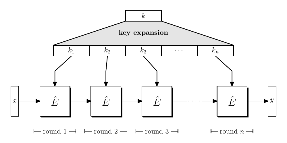
Since $\hat{E}(k,x) \to y$, which is a round function, we have $|x| = |y|$, where $n$ times applied $\hat{E}$ constructed a PRF or PRP.

All info comes from David Wu’s Lecture and Boneh-Shoup Book.

This note will be focusing on PRG security, PRF and Block Cipher.

Claim: If PRGs with non-trivial stretch ($n > \lambda$) exists, then $P\neq NP$.

Suppose $G :\lbrace 0,1\rbrace^\lambda \to \lbrace 0,1\rbrace^n$ is a secure PRG, consider the decision problem: on input $t\in \lbrace 0, 1\rbrace ^n$, does there exist $s \in \lbrace 0,1\rbrace^\lambda$ such that $ t = G(s)$.

The reverse search of $G$ is in $NP$. If $G$ is secure, then no poly-time algorithm can solve this problem.

If there is a poly-time algorithm for the problem, it breaks PRG in advantage of $1 - \dfrac{1}{2^{n-\lambda}} > \dfrac{1}{2}$ since $n>\lambda$.

All info comes from David Wu’s Lecture and Boneh-Shoup Book.

This note will be focusing mainly on perfect security, semantics security and PRG (Pseudo Random Generator).

The overall goal of cryptography is to secure communication over untrusted network. Two things must be achieved:

• Confidentiality: No one can eavesdrop the communication
• Integrity: No one can tamper with communication

Perfect Security

A cipher $(Enc, Dec)$ satisfies perfect secure if $\forall m_0, m_1 \in M$ and $\forall c\in C$, $\Pr[k\overset{R}{\longleftarrow} K: Enc(k, m_0) = c] = \Pr[k\overset{R}{\longleftarrow} K:Enc(k,m_1) = c]$.

$k$ in two $\Pr$ might mean different $k$, the $\Pr$ just indicate the possibility of $\dfrac{\text{number of }k\text{ that }Enc(k, m) = c}{|K|}$.

OTP is Perfect Secure

For every fixed $m = \lbrace 0, 1\rbrace^n$ there is $k, c = \lbrace 0, 1\rbrace^n$ uniquely paired that $m \oplus k = c$.

Considering perfect security definition, only one $k$ can encrypt $m$ to $c$. Thus $\Pr = \dfrac{1}{|K|} = \dfrac{1}{2^n}$ and equation is satisfied.

Shannon “Bad News” Theorem

If a cipher is perfect secure, then $|K| \ge |M|$.

Assume $|K| < |M|$, we want to show it is not perfect secure. Let $k_0 \in K$ and $m_0 \in M$, then $c \leftarrow Enc(k_0, m_0)$. Let $S = \lbrace Dec(k, c): k \in K\rbrace$, we can see $|S| \le |K| < |M|$.

We can see that $\Pr\lbrack k \overset{R}{\longleftarrow} K: Enc(k, m_0) = c\rbrack > 0$, if we choose $m_1 \in M \backslash S$, then $\not\exists k \in K: Enc(k, m_1) = c$. Thus it is not perfect secure. $\square$

Isomorphism or invertible map will be discussed in this chapter.

Isomorphism as Invertible Map

The crucial part of such map property is that an inverse map exists that $f: A \longrightarrow B$ has a $g$ inverse that satisfies $g \circ f \equiv 1_A$ and $f \circ g \equiv 1_B$.

A similarity between two collections can be given by choosing a map, which maps each element from the first one to the second one.

Sets, maps and the map composition will be talked about in this note.

If we ignore the value of conditions by treating if or while statements as nondeterministic choices between two branches, we call these analyses as path insensitive analysis.

Path sensitive analysis is used to increase pessimistic accuracy of path insensitive analysis.

Interval analysis can be used in integer representation or array bound check. This would involve widening and narrowing.

A lattice of intervals is defined as $\text{Interval} \triangleq \text{lift}(\lbrace \lbrack l,h\rbrack \mid l,h\in\mathbb{Z} \wedge l \leq h\rbrace)$. The partial order is defined as $\lbrack l_1,h_1\rbrack \sqsubseteq \lbrack l_2,h_2\rbrack \iff l_2 \leq l_1 \wedge h_1 \le h_2$.

The top is defined to be $\lbrack -\infty,+\infty\rbrack$ and the bottom is defined as $\bot$, which means no integer. Since the chain of partial order can have infinite length, the lattice itself has infinite height.

The total lattice for a program point is $L = \text{Vars}\to \text{Interval}$, which provides bounds for each integer value.

The constraint rules are listed as
$$
\begin{aligned}
& & & JOIN(v) = \bigsqcup_{w\in pred(v)}\lbrack \lbrack w\rbrack \rbrack \newline
\lbrack\lbrack X = E\rbrack\rbrack &\phantom{:::} \lbrack\lbrack v\rbrack\rbrack &=& JOIN(v) \lbrack X \mapsto \text{eval}(JOIN(v), E)\rbrack\newline
& & & \text{eval}(\sigma, X) = \sigma(X)\newline
& & & \text{eval}(\sigma, I) = \lbrack I, I\rbrack\newline
& & & \text{eval}(\sigma, \text{input}) = \lbrack -\infty, \infty\rbrack\newline
& & & \text{eval}(\sigma, E_1\ op\ E_2) = \hat{op}(\text{eval}(\sigma, E_1), \text{eval}(\sigma, E_2))\newline
& & & \hat{op}(\lbrack l_1,r_1\rbrack, \lbrack l_2,r_2\rbrack) = \lbrack \min_{x\in \lbrack l_1,r_1\rbrack, y\in \lbrack l_2,r_2\rbrack} x\ op\ y, \max_{x\in \lbrack l_1,r_1\rbrack, y\in \lbrack l_2,r_2\rbrack }x\ op\ y\rbrack \newline
& \phantom{:::}\lbrack\lbrack v\rbrack\rbrack &=& JOIN(v)\newline
& \lbrack \lbrack exit\rbrack\rbrack &=& \varnothing
\end{aligned}
$$
The fixed-point problem we previously discussed is only restricted in lattice with finite height. New fixed-point algorithm is needed in practical space.

More flow sensitive analysis (data flow analysis) on the way

This part will take notes about Lattice Theory.

Appetizer: Sign analysis can be done by first construct a lattice with elements $\lbrace +,-,0,\top,\bot\rbrace$ with each parts’ meaning:

• $+, -, 0$ stand for integer value signs
• $\top$ stands for any integer values while $\bot$ means empty set of integer values.

$$
\begin{array}{ccccc}
& & \top& & \newline
& \swarrow & \downarrow & \searrow \newline
& + & 0 &- \newline
& \searrow & \downarrow & \swarrow \newline
& &\bot
\end{array}
$$

All info comes from Manuel’s slides on Lecture 4.

Intros on Hash Functions

What if we want some high-level of fingerprint that can be built from any data, with a tiny change in data cause radical impact on the whole fingerprint.

All info comes from Manuel’s slides on Lecture 3.

Public-Key Cryptosystem

Encryption depends on a public key $K$ and decryption depends on a secret key $K’$.

Finding $K’$ when knowing $K$ is computationally infeasible.

All info comes from Manuel’s slides on Lecture 2.

Block Cipher

A block cipher is composed of 2 co-inverse functions:
$$
\begin{aligned}
E:\lbrace 0,1\rbrace^n\times\lbrace0,1\rbrace^k&\to\lbrace 0,1\rbrace^n& D:\lbrace 0,1\rbrace^n\times\lbrace0,1\rbrace^k&\to\lbrace 0,1\rbrace^n\\
(P,K)&\mapsto C&(C,K)&\mapsto P
\end{aligned}
$$
where $n,k$ means the size of a block and key respectively.

The goal is that given a key $K$ and design an invertible function $E$ whose output cannot be distinguished from a random permutation over $\lbrace 0, 1\rbrace^n$.

All info comes from Manuel’s slides on Lecture 1.

Please refer this link from page 177 to 184.

Intros on System FPC and Recursive Types

FPC is a language with products, sums, partial functions, and recursive types.

Recursive types are solutions to type equations $t\cong\tau$ where there is no restriction on $t$ occurrence in $\tau$. Equivalently, it is a fixed point up to isomorphism of associated unrestricted type operator $t.\tau$. When removing the restriction on type operator, we may see the solution satisfies $t\cong t\rightharpoonup t$, which describes a type is isomorphic to the type of partial function defined on itself.

Types are not sets: they classify computable functions not arbitrary functions. With types we may solve such type equations. The penalty is that we must admit non-termination. For one thing, type equations involving functions have solutions only if the functions involved are partial.

A benefit of working in the setting of partial functions is that type operations have unique solutions (up to isomorphism). But what about the inductive/coinductive type as solution to same type equation? This turns out that based on fixed dynamics, be it lazy or eager:

• Under a lazy dynamics, recursive types have a coinductive flavor, and inductive analogs are inaccessible.
• Under an eager dynamics, recursive types have an inductive flavor, but coinductive analogs are accessible as well.

他依然向往着长岛的雪，依然向往着潘帕斯的风吟鸟唱。很久以后我才知道，长岛是没有雪的。

我想先尝试聊聊两部电影，一部是“Paris, Texas”（德州巴黎），还有一部是“Her”（她）。

但是在打草稿时发现，记忆和情绪蔓延开让它四不像，既不像影评又不像笔记，我又不舍得把它们删掉。因此这篇文章简直在胡说八道（笑），满是一个肉欲和精神骚动得不到慰藉的死宅男的意淫。

原先的计划是写电影如何通过色彩来传达情绪，但我觉得豆瓣上已经存在了无数类似的文字，我也并非专业的学院派，水平有限。我寻思着把每个镜头每个像素点铺平碾碎理顺，它们就被亵渎了。总有些东西是要留在符号体系之外，不去解释的。暴殄天物的后果就是再也无法被触动，之后的情人节也就得找新的电影，我也懒得找，年年有此日岁岁有此朝。

思忖了半天，我还是适合当一个吹水的说书人。（就把我想成上海夏天弄堂口背心短裤人字拖的搓麻将爷叔）

于是在风和日丽的一天，我看着原本的草稿，不再有原先心跳的悸动，气息渐平，指尖不颤。讲张三写李四，从一件事聊到另一件事。

孤独是一种会上瘾的情绪，让人沉沦。我试过酒，试过更糟的东西，都不能与之比肩。

那么当我们谈论孤独的时候，我们在谈论什么？

话说回来我还没有一个像样的卷首，感觉不太像样。我建立这个博客是为了给自己的想法留一个栖身之所，即使他们可能幼稚又愚蠢。没有一个卷首语，似乎就没有一个正式的开始，鄙弃仪式性的我都看不下去了。

Please refer this link from page 167 to 176.

Intros on General Recursion and Fixpoint

System T is introduced as a basis for discussing total computations, those for which the type systems guarantees termination.

Language M generalizes T to admit inductive and coinductive types, while preserving totality.

PCF will be introduced here as a basis for discussing partial computations, those may not terminate while evaluated, even if they are well typed.

Seems like a disadvantage, it admits greater expressive power than is possible in T.

The source of partiality in PCF is the concept of general recursion, permitting solution of equations between expressions. We can see the advantages and disadvantages clearly that:

• The price of admitting solutions to all such equations is that the computation may not terminate: the solution of some equations may be divergent or undefined.
• The advantage is that termination proof need not be embedded into the code, resulting in short code.

A solution to such a system of equations is a fixed point of an associated functional (higher-order function).

This part is not shown on PFPL preview version.

Intros and Examples

Concept of type quantification leads to consideration of quantification over type constructors, which are functions mapping types to types.

For example, take queue here, the abstract type constructor can be expressed by existential type $\exists q::\text{T}\to\text{T}.\sigma$, where $\sigma$ is labeled tuple type and existential type $q\lbrack t\rbrack$ quantifies over kind $\text{T}\to\text{T}$.
$$
\begin{matrix}
\langle&&\text{emp}&&\hookrightarrow&&\forall t::\text{T}.t,&&\\
&&\text{ins}&&\hookrightarrow&&\forall t::\text{T}.t\times q\lbrack t\rbrack\to q\lbrack t\rbrack,&&\\
&&\text{rem}&&\hookrightarrow&&\forall t::\text{T}.q\lbrack t\rbrack\to(t\times q\lbrack t\rbrack)\space\text{opt}&&\rangle
\end{matrix}
$$
Language $\text{F}_\omega$ enriches language F with universal and existential quantification over kinds. This extension accounts for definitional equality of constructors.

Please refer this link from page 151 to 158.

Data Abstraction and Existential Types

Data abstraction has great importance for structuring programs. The main idea is to introduce an interface that serves as a contract between the client and implementor of an abstract type. The interface specifies

• what client relies on to continue its work.
• what implementor must provide to satisfy the contract.

The interface serves to isolate the client from implementor so that they can be developed isolated. This property is called representation independence for abstract type.

Existential types are introduced in extending language F in formalizing data abstraction.

• Interfaces are existential types that provide a collection of operations on unspecified, or abstract types.
• Implementations are packages, introduction forms of existential types.
• Clients are uses of corresponding elimination form.

Please refer this link from page 141 to 149.

From Monomorphic to Polymorphic

So far we are dealing with monomorphic languages since every expression has a unique type. If we want a same behavior over different types, different programs will have to be created.

The expression patterns codify generic (type-independent) behaviors that are shared by all instances of the pattern. Such generic expressions are polymorphic.